I noticed the cleaning guy at work looks like Ron Jeremy in the face. I mentioned it to him. He said, most people thought he looked like Danny Devito.

I said, oh yeah! You have Ron Jeremy’s head on Danny Devito’s body. Then I asked AI what it would look like if you put Ron Jeremy’s head on Danny Devito’s body. It answered, It would look like the guy that played the Penguin on Batman.

Then I asked AI to create a picture of Ron Jeremy’s head on Danny Devito’s body.

OLS

> fit.ols<-glm(usarea ~ lmhhinc   + lpop + pnhblk + punemp + pvac  + ph70 + lmhval +

+                 phnew + phisp, data = philly2)

> summary(fit.ols)

Call:

glm(formula = usarea ~ lmhhinc + lpop + pnhblk + punemp + pvac + 

    ph70 + lmhval + phnew + phisp, data = philly2)

Coefficients:

            Estimate Std. Error t value Pr(>|t|)    

(Intercept)  534.491    164.270   3.254  0.00124 ** 

lmhhinc        2.462     12.176   0.202  0.83990    

lpop          -1.344      6.338  -0.212  0.83216    

pnhblk        21.158     18.077   1.170  0.24260    

punemp        -5.097     63.645  -0.080  0.93622    

pvac         371.699     58.427   6.362 5.96e-10 ***

ph70         -79.691     35.535  -2.243  0.02552 *  

lmhval       -45.668     10.458  -4.367 1.64e-05 ***

phnew         17.958    319.042   0.056  0.95514    

phisp        -56.308     30.695  -1.834  0.06741 .  

—

Signif. codes:  0 ‘***’ 0.001 ‘**’ 0.01 ‘*’ 0.05 ‘.’ 0.1 ‘ ’ 1

(Dispersion parameter for gaussian family taken to be 4829.927)

    Null deviance: 2938287  on 375  degrees of freedom

Residual deviance: 1767753  on 366  degrees of freedom

AIC: 4268.4

Number of Fisher Scoring iterations: 2

GWR

gwr.fit1<-gwr(usarea ~ lmhhinc   + lpop + pnhblk + punemp + pvac  + ph70 + lmhval +phnew + phisp, data = philly2.sp, bandwidth = gwr.b1, se.fit=T, hatmatrix=T)

> gwr.fit1

Call:

gwr(formula = usarea ~ lmhhinc + lpop + pnhblk + punemp + pvac + 

    ph70 + lmhval + phnew + phisp, data = philly2.sp, bandwidth = gwr.b1, 

    hatmatrix = T, se.fit = T)

Kernel function: gwr.Gauss 

Fixed bandwidth: 1322.708 

Summary of GWR coefficient estimates at data points:

                   Min.    1st Qu.     Median    3rd Qu.       Max.   Global

X.Intercept. -1574.4098   -53.8875    88.4952   472.7282  3092.1466 534.4908

lmhhinc       -151.0306    -7.0538     3.2205    22.3099   120.2753   2.4616

lpop           -76.6700     1.1576     7.2067    20.4788   109.5747  -1.3441

pnhblk        -124.9781    -2.0948    44.5163   100.0885   490.8730  21.1576

punemp        -627.4200  -150.5909   -17.8892    69.6271   752.1507  -5.0966

pvac         -1329.2458     2.5473   165.4452   343.9353  1108.9034 371.6993

ph70         -1028.8902  -161.7810   -43.4011    -8.2491   144.6265 -79.6910

lmhval        -178.5925   -70.3725   -26.7389    -3.7657    89.1748 -45.6676

phnew        -3747.6137  -484.6544    54.6557   734.6135  6434.5611  17.9575

phisp         -313.3416   -24.9975     4.8295   117.2091  1533.6439 -56.3076

Number of data points: 376 

Effective number of parameters (residual: 2traceS – traceS’S): 220.8092 

Effective degrees of freedom (residual: 2traceS – traceS’S): 155.1908 

Sigma (residual: 2traceS – traceS’S): 59.06332 

Effective number of parameters (model: traceS): 178.5045 

Effective degrees of freedom (model: traceS): 197.4955 

Sigma (model: traceS): 52.3567 

Sigma (ML): 37.9452 

AICc (GWR p. 61, eq 2.33; p. 96, eq. 4.21): 4491.91 

AIC (GWR p. 96, eq. 4.22): 3979.926 

Residual sum of squares: 541379.3 

Quasi-global R2: 0.81575

> gwr.b2<-gwr.sel(usarea ~ lmhhinc   + lpop + pnhblk + punemp + pvac  + ph70 + lmhval +phnew + phisp, data = philly2.sp, gweight = gwr.bisquare)

> gwr.fit2<-gwr(usarea ~ lmhhinc   + lpop + pnhblk + punemp + pvac  + ph70 + lmhval +phnew + phisp, data = philly2.sp, bandwidth = gwr.b2, gweight = gwr.bisquare, se.fit=T, hatmatrix=T)

> gwr.fit2

Call:

gwr(formula = usarea ~ lmhhinc + lpop + pnhblk + punemp + pvac + 

    ph70 + lmhval + phnew + phisp, data = philly2.sp, bandwidth = gwr.b2, 

    gweight = gwr.bisquare, hatmatrix = T, se.fit = T)

Kernel function: gwr.bisquare 

Fixed bandwidth: 5092.898 

Summary of GWR coefficient estimates at data points:

                   Min.    1st Qu.     Median    3rd Qu.       Max.   Global

X.Intercept.  -649.3890    -5.7699   134.6249   512.9574  2336.5957 534.4908

lmhhinc       -180.3145    -4.4545     1.7487    13.7554    68.2914   2.4616

lpop           -49.1608     1.2314     6.3430    19.0823    69.7005  -1.3441

pnhblk        -106.4233     1.3658    41.0256    96.5291   285.2134  21.1576

punemp        -397.5988  -143.8982    -6.2685    57.4553   729.4700  -5.0966

pvac          -757.5534     8.8245   209.8576   370.7793   650.3669 371.6993

ph70          -643.0070  -207.9799   -66.3040   -19.8028   142.9682 -79.6910

lmhval        -150.2726   -69.5496   -34.8198    -6.7118   107.7625 -45.6676

phnew        -1844.6086  -418.1211    19.6153   509.9117  7421.2055  17.9575

phisp         -221.0604   -26.5670    -7.5865    84.2566  1418.3152 -56.3076

Number of data points: 376 

Effective number of parameters (residual: 2traceS – traceS’S): 132.4964 

Effective degrees of freedom (residual: 2traceS – traceS’S): 243.5036 

Sigma (residual: 2traceS – traceS’S): 62.2312 

Effective number of parameters (model: traceS): 107.6713 

Effective degrees of freedom (model: traceS): 268.3287 

Sigma (model: traceS): 59.2826 

Sigma (ML): 50.0803 

AICc (GWR p. 61, eq 2.33; p. 96, eq. 4.21): 4316.932 

AIC (GWR p. 96, eq. 4.22): 4117.761 

Residual sum of squares: 943021.6 

Quasi-global R2: 0.6790573

gwr.b3<-gwr.sel(usarea ~ lmhhinc   + lpop + pnhblk + punemp + pvac  + ph70 +

                    lmhval + phnew + phisp, data = philly2.sp, adapt = TRUE)

gwr.fit3<-gwr(usarea ~ lmhhinc   + lpop + pnhblk + punemp + pvac  + ph70 + lmhval +

+                  phnew + phisp, data = philly2.sp, adapt=gwr.b3, se.fit=T, hatmatrix=T)

> gwr.fit3

Call:

gwr(formula = usarea ~ lmhhinc + lpop + pnhblk + punemp + pvac + 

    ph70 + lmhval + phnew + phisp, data = philly2.sp, adapt = gwr.b3, 

    hatmatrix = T, se.fit = T)

Kernel function: gwr.Gauss 

Adaptive quantile: 0.02491844 (about 9 of 376 data points)

Summary of GWR coefficient estimates at data points:

                    Min.     1st Qu.      Median     3rd Qu.        Max.   Global

X.Intercept. -1413.25718     2.04814   150.67770   593.38119  2856.09861 534.4908

lmhhinc        -77.30238    -6.62505     2.08877    20.59832   121.03243   2.4616

lpop           -71.53993     0.32328     6.55222    19.42020    93.59455  -1.3441

pnhblk        -139.33868    -0.35274    39.43998   102.07286   462.87992  21.1576

punemp        -592.27650  -109.64202    -3.93096    63.56270   623.38186  -5.0966

pvac         -1410.12965    11.95427   193.34738   350.39251  1047.77143 371.6993

ph70          -975.65611  -190.62161   -67.38336   -13.17506   137.47857 -79.6910

lmhval        -185.48730   -73.39044   -36.70912    -7.56967    48.91389 -45.6676

phnew        -2570.54553  -577.37945    29.21937   654.40082  4045.23829  17.9575

phisp         -182.91660   -29.72723    -7.23980    65.71058   771.29484 -56.3076

Number of data points: 376 

Effective number of parameters (residual: 2traceS – traceS’S): 177.8408 

Effective degrees of freedom (residual: 2traceS – traceS’S): 198.1592 

Sigma (residual: 2traceS – traceS’S): 54.21695 

Effective number of parameters (model: traceS): 135.2358 

Effective degrees of freedom (model: traceS): 240.7642 

Sigma (model: traceS): 49.18654 

Sigma (ML): 39.35938 

AICc (GWR p. 61, eq 2.33; p. 96, eq. 4.21): 4258.02 

AIC (GWR p. 96, eq. 4.22): 3964.174 

Residual sum of squares: 582484.4 

Quasi-global R2: 0.8017605

> gwr.fit1$bandwidth

[1] 1322.708

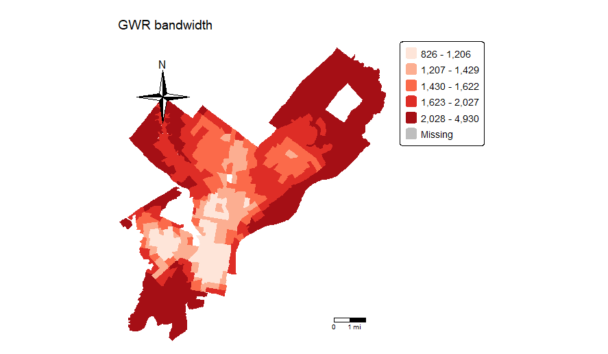
> philly2$bwadapt <- gwr.fit3$bandwidth

> tm_shape(philly2, unit = “mi”) +

+    tm_polygons(col = “bwadapt”, style = “quantile”,palette = “Reds”,

+                border.alpha = 0, title = “”) +

+    tm_scale_bar(breaks = c(0, 1, 2), size = 1, position = c(“right”, “bottom”)) +

+    tm_compass(type = “4star”, position = c(“left”, “top”)) +

+    tm_layout(main.title = “GWR bandwidth”,  main.title.size = 0.95, frame = FALSE, legend.outside = TRUE)

I have been harassed without provocation or warrant by a crew of Vice detectives out of the Pacific Division. The D2’s name is Edward Acosta. He supervises 2 D1’s and he has employed his own son and the son of one of the D1s he supervises to assist in attacking me. The campaign of terror started in May and has continued until this week. I can present a case to you and supply you with plenty of evidence to prove my claim. They are transphobic. I have been targeted as the result of being transgender. I’m attempting to discern the best way to communicate this information to initiate an investigation with Los Angeles Police Department Internal Affairs.

Thank you,

Barbie