Ordinary Least Squares vs. Geographically Weighted Regression Model for Philadelphia Building Code Violations Using R

OLS

> fit.ols<-glm(usarea ~ lmhhinc   + lpop + pnhblk + punemp + pvac  + ph70 + lmhval +

+                 phnew + phisp, data = philly2)

> summary(fit.ols)

Call:

glm(formula = usarea ~ lmhhinc + lpop + pnhblk + punemp + pvac + 

    ph70 + lmhval + phnew + phisp, data = philly2)

Coefficients:

            Estimate Std. Error t value Pr(>|t|)    

(Intercept)  534.491    164.270   3.254  0.00124 ** 

lmhhinc        2.462     12.176   0.202  0.83990    

lpop          -1.344      6.338  -0.212  0.83216    

pnhblk        21.158     18.077   1.170  0.24260    

punemp        -5.097     63.645  -0.080  0.93622    

pvac         371.699     58.427   6.362 5.96e-10 ***

ph70         -79.691     35.535  -2.243  0.02552 *  

lmhval       -45.668     10.458  -4.367 1.64e-05 ***

phnew         17.958    319.042   0.056  0.95514    

phisp        -56.308     30.695  -1.834  0.06741 .  

—

Signif. codes:  0 ‘***’ 0.001 ‘**’ 0.01 ‘*’ 0.05 ‘.’ 0.1 ‘ ’ 1

(Dispersion parameter for gaussian family taken to be 4829.927)

    Null deviance: 2938287  on 375  degrees of freedom

Residual deviance: 1767753  on 366  degrees of freedom

AIC: 4268.4

Number of Fisher Scoring iterations: 2

GWR

gwr.fit1<-gwr(usarea ~ lmhhinc   + lpop + pnhblk + punemp + pvac  + ph70 + lmhval +phnew + phisp, data = philly2.sp, bandwidth = gwr.b1, se.fit=T, hatmatrix=T)

> gwr.fit1

Call:

gwr(formula = usarea ~ lmhhinc + lpop + pnhblk + punemp + pvac + 

    ph70 + lmhval + phnew + phisp, data = philly2.sp, bandwidth = gwr.b1, 

    hatmatrix = T, se.fit = T)

Kernel function: gwr.Gauss 

Fixed bandwidth: 1322.708 

Summary of GWR coefficient estimates at data points:

                   Min.    1st Qu.     Median    3rd Qu.       Max.   Global

X.Intercept. -1574.4098   -53.8875    88.4952   472.7282  3092.1466 534.4908

lmhhinc       -151.0306    -7.0538     3.2205    22.3099   120.2753   2.4616

lpop           -76.6700     1.1576     7.2067    20.4788   109.5747  -1.3441

pnhblk        -124.9781    -2.0948    44.5163   100.0885   490.8730  21.1576

punemp        -627.4200  -150.5909   -17.8892    69.6271   752.1507  -5.0966

pvac         -1329.2458     2.5473   165.4452   343.9353  1108.9034 371.6993

ph70         -1028.8902  -161.7810   -43.4011    -8.2491   144.6265 -79.6910

lmhval        -178.5925   -70.3725   -26.7389    -3.7657    89.1748 -45.6676

phnew        -3747.6137  -484.6544    54.6557   734.6135  6434.5611  17.9575

phisp         -313.3416   -24.9975     4.8295   117.2091  1533.6439 -56.3076

Number of data points: 376 

Effective number of parameters (residual: 2traceS – traceS’S): 220.8092 

Effective degrees of freedom (residual: 2traceS – traceS’S): 155.1908 

Sigma (residual: 2traceS – traceS’S): 59.06332 

Effective number of parameters (model: traceS): 178.5045 

Effective degrees of freedom (model: traceS): 197.4955 

Sigma (model: traceS): 52.3567 

Sigma (ML): 37.9452 

AICc (GWR p. 61, eq 2.33; p. 96, eq. 4.21): 4491.91 

AIC (GWR p. 96, eq. 4.22): 3979.926 

Residual sum of squares: 541379.3 

Quasi-global R2: 0.81575

> gwr.b2<-gwr.sel(usarea ~ lmhhinc   + lpop + pnhblk + punemp + pvac  + ph70 + lmhval +phnew + phisp, data = philly2.sp, gweight = gwr.bisquare)

> gwr.fit2<-gwr(usarea ~ lmhhinc   + lpop + pnhblk + punemp + pvac  + ph70 + lmhval +phnew + phisp, data = philly2.sp, bandwidth = gwr.b2, gweight = gwr.bisquare, se.fit=T, hatmatrix=T)

> gwr.fit2

Call:

gwr(formula = usarea ~ lmhhinc + lpop + pnhblk + punemp + pvac + 

    ph70 + lmhval + phnew + phisp, data = philly2.sp, bandwidth = gwr.b2, 

    gweight = gwr.bisquare, hatmatrix = T, se.fit = T)

Kernel function: gwr.bisquare 

Fixed bandwidth: 5092.898 

Summary of GWR coefficient estimates at data points:

                   Min.    1st Qu.     Median    3rd Qu.       Max.   Global

X.Intercept.  -649.3890    -5.7699   134.6249   512.9574  2336.5957 534.4908

lmhhinc       -180.3145    -4.4545     1.7487    13.7554    68.2914   2.4616

lpop           -49.1608     1.2314     6.3430    19.0823    69.7005  -1.3441

pnhblk        -106.4233     1.3658    41.0256    96.5291   285.2134  21.1576

punemp        -397.5988  -143.8982    -6.2685    57.4553   729.4700  -5.0966

pvac          -757.5534     8.8245   209.8576   370.7793   650.3669 371.6993

ph70          -643.0070  -207.9799   -66.3040   -19.8028   142.9682 -79.6910

lmhval        -150.2726   -69.5496   -34.8198    -6.7118   107.7625 -45.6676

phnew        -1844.6086  -418.1211    19.6153   509.9117  7421.2055  17.9575

phisp         -221.0604   -26.5670    -7.5865    84.2566  1418.3152 -56.3076

Number of data points: 376 

Effective number of parameters (residual: 2traceS – traceS’S): 132.4964 

Effective degrees of freedom (residual: 2traceS – traceS’S): 243.5036 

Sigma (residual: 2traceS – traceS’S): 62.2312 

Effective number of parameters (model: traceS): 107.6713 

Effective degrees of freedom (model: traceS): 268.3287 

Sigma (model: traceS): 59.2826 

Sigma (ML): 50.0803 

AICc (GWR p. 61, eq 2.33; p. 96, eq. 4.21): 4316.932 

AIC (GWR p. 96, eq. 4.22): 4117.761 

Residual sum of squares: 943021.6 

Quasi-global R2: 0.6790573

gwr.b3<-gwr.sel(usarea ~ lmhhinc   + lpop + pnhblk + punemp + pvac  + ph70 +

                    lmhval + phnew + phisp, data = philly2.sp, adapt = TRUE)

gwr.fit3<-gwr(usarea ~ lmhhinc   + lpop + pnhblk + punemp + pvac  + ph70 + lmhval +

+                  phnew + phisp, data = philly2.sp, adapt=gwr.b3, se.fit=T, hatmatrix=T)

> gwr.fit3

Call:

gwr(formula = usarea ~ lmhhinc + lpop + pnhblk + punemp + pvac + 

    ph70 + lmhval + phnew + phisp, data = philly2.sp, adapt = gwr.b3, 

    hatmatrix = T, se.fit = T)

Kernel function: gwr.Gauss 

Adaptive quantile: 0.02491844 (about 9 of 376 data points)

Summary of GWR coefficient estimates at data points:

                    Min.     1st Qu.      Median     3rd Qu.        Max.   Global

X.Intercept. -1413.25718     2.04814   150.67770   593.38119  2856.09861 534.4908

lmhhinc        -77.30238    -6.62505     2.08877    20.59832   121.03243   2.4616

lpop           -71.53993     0.32328     6.55222    19.42020    93.59455  -1.3441

pnhblk        -139.33868    -0.35274    39.43998   102.07286   462.87992  21.1576

punemp        -592.27650  -109.64202    -3.93096    63.56270   623.38186  -5.0966

pvac         -1410.12965    11.95427   193.34738   350.39251  1047.77143 371.6993

ph70          -975.65611  -190.62161   -67.38336   -13.17506   137.47857 -79.6910

lmhval        -185.48730   -73.39044   -36.70912    -7.56967    48.91389 -45.6676

phnew        -2570.54553  -577.37945    29.21937   654.40082  4045.23829  17.9575

phisp         -182.91660   -29.72723    -7.23980    65.71058   771.29484 -56.3076

Number of data points: 376 

Effective number of parameters (residual: 2traceS – traceS’S): 177.8408 

Effective degrees of freedom (residual: 2traceS – traceS’S): 198.1592 

Sigma (residual: 2traceS – traceS’S): 54.21695 

Effective number of parameters (model: traceS): 135.2358 

Effective degrees of freedom (model: traceS): 240.7642 

Sigma (model: traceS): 49.18654 

Sigma (ML): 39.35938 

AICc (GWR p. 61, eq 2.33; p. 96, eq. 4.21): 4258.02 

AIC (GWR p. 96, eq. 4.22): 3964.174 

Residual sum of squares: 582484.4 

Quasi-global R2: 0.8017605

> gwr.fit1$bandwidth

[1] 1322.708

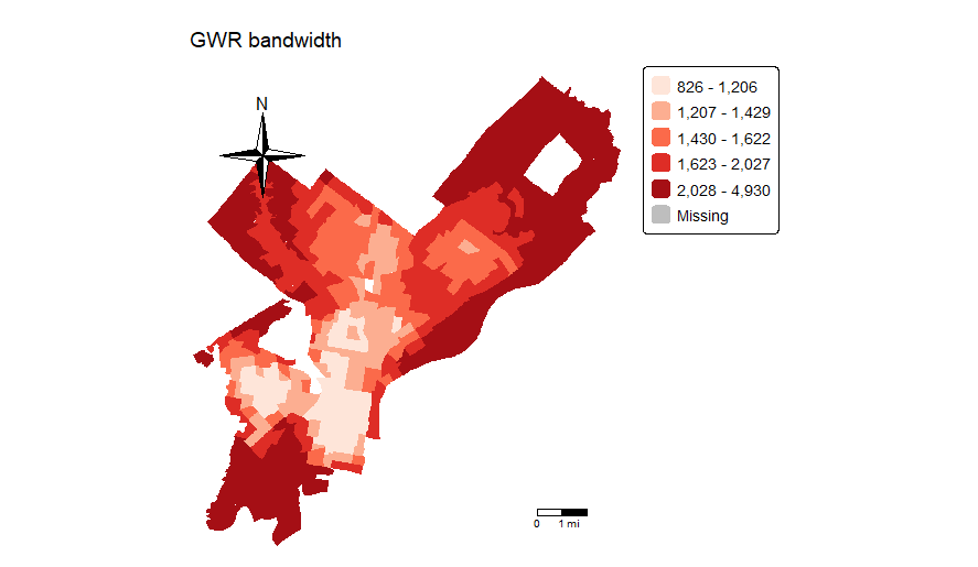
> philly2$bwadapt <- gwr.fit3$bandwidth

> tm_shape(philly2, unit = “mi”) +

+    tm_polygons(col = “bwadapt”, style = “quantile”,palette = “Reds”,

+                border.alpha = 0, title = “”) +

+    tm_scale_bar(breaks = c(0, 1, 2), size = 1, position = c(“right”, “bottom”)) +

+    tm_compass(type = “4star”, position = c(“left”, “top”)) +

+    tm_layout(main.title = “GWR bandwidth”,  main.title.size = 0.95, frame = FALSE, legend.outside = TRUE)